Tsallis entropy, one dial at a time

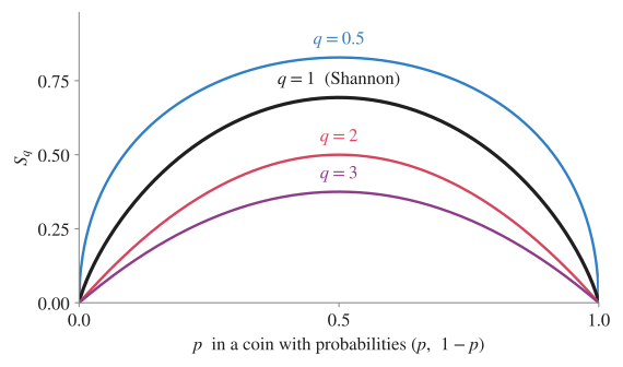
Most of the statistics in modern machine learning (softmax, cross-entropy, the Gaussian, the KL divergence) descends from one quantity, the Shannon entropy $S = -\sum_i p_i \ln p_i$, and from one assumption hidden inside it: that information is additive. In 1988 Constantino Tsallis proposed a one-parameter generalisation,

$$S_q(p) = \frac{1 - \sum_i p_i^{\,q}}{q - 1}, \qquad \lim_{q \to 1} S_q(p) = -\sum_i p_i \ln p_i .$$

The entropic index $q$ is a dial. Values $q < 1$ give more weight to rare events and $q > 1$ to frequent ones, and at $q = 1$ everything collapses back to the standard theory. This note follows our perspective paper, Perspectives on Tsallis Statistics for Artificial Intelligence, and keeps only the essentials.

Non-additive, so that it can be extensive

For two independent systems the Tsallis entropy does not simply add:

$$S_q(A \cup B) = S_q(A) + S_q(B) + (1 - q)\, S_q(A)\, S_q(B).$$

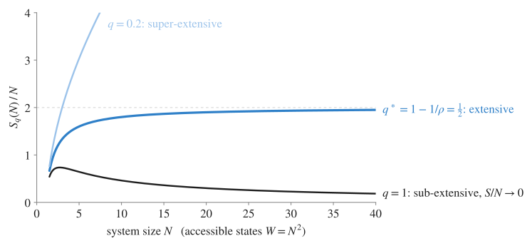
This looks like a defect until one separates two properties that are easy to conflate. Additivity belongs to the entropy functional. Extensivity, $S(N) \propto N$, belongs to a physical system. They coincide only when the parts are weakly correlated. If strong correlations make the number of accessible states grow as a power law, $W(N) \propto N^{\rho}$, then the Shannon entropy $\ln W$ grows only logarithmically, while $S_q = \ln_q W$ is extensive for exactly one index, $q^\ast = 1 - 1/\rho$.

The q-algebra

The theory rests on a deformed logarithm and its inverse,

$$\ln_q x = \frac{x^{1-q} - 1}{1 - q}, \qquad \exp_q(x) = \big[\,1 + (1-q)\,x\,\big]_+^{\frac{1}{1-q}},$$

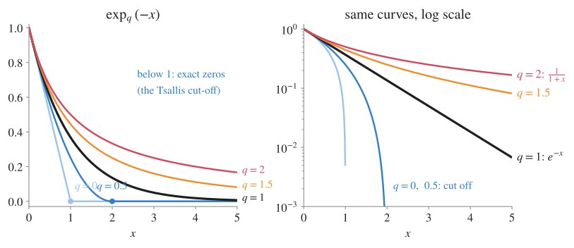
where $[y]_+ = \max(y, 0)$. That small bracket, the Tsallis cut-off, carries most of the consequences. For $q < 1$ the q-exponential reaches exactly zero at a finite point, which is the source of sparsity. For $q > 1$ it decays as a power law, which is the source of heavy tails. Maximising $S_q$ under normalisation and an energy constraint replaces the Boltzmann weight $e^{-\beta \varepsilon}$ by $\exp_q(-\beta \varepsilon)$.

q-Gaussians

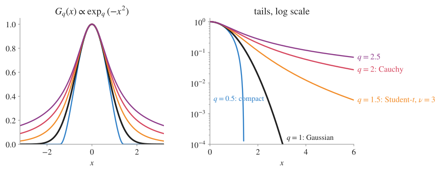
Maximising $S_q$ at fixed (generalised) variance gives the q-Gaussian, $G_q(x) \propto \exp_q(-\beta x^2)$, a single family that moves continuously between familiar distributions:

$q$	distribution	tails
$< 1$	compact support	none
$1$	Gaussian	light
$(1, 3)$	Student-$t$, $\nu = \frac{3 - q}{q - 1}$	power law
$2$	Cauchy	power law

The variance is finite only for $q < 5/3$. Just as the Gaussian is the limit of sums of independent variables, q-Gaussians are the limits of sums of strongly correlated ones (the q-central limit theorem). Many models that are called "robust" or "heavy-tailed" are q-Gaussian models in disguise.

Where q comes from

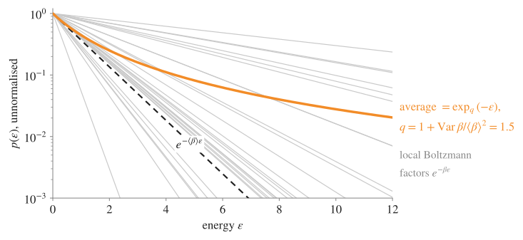
Where does the value of $q$ come from? Superstatistics gives the clearest answer. Suppose a system is locally Boltzmann, $p(\varepsilon \mid \beta) \propto e^{-\beta \varepsilon}$, but its inverse temperature $\beta$ fluctuates slowly from place to place. If $\beta$ is gamma-distributed, the average is exactly a q-exponential, with

$$q = 1 + \frac{\operatorname{Var}\beta}{\langle \beta \rangle^{2}} .$$

So $q - 1$ measures heterogeneity. Machine learning is full of such mixtures: mini-batches sample different local losses, dropout and ensembles average over parameters, and mixture-of-experts layers combine components working at different scales.

Sparse attention is a Tsallis softmax

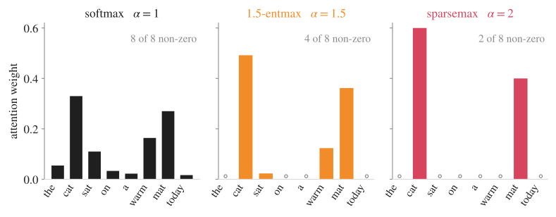
The softmax solves an entropy-regularised problem, $\operatorname{softmax}(z) = \arg\max_{p \in \Delta}\, p^\top z + H(p)$. Shannon entropy is infinitely steep at the edge of the simplex, so every option keeps some probability. Swapping $H$ for the Tsallis entropy gives α-entmax, with $\alpha$ playing the role of $q$:

$$\alpha\text{-entmax}(z) = \arg\max_{p \in \Delta}\; p^\top z + S_\alpha(p).$$

At $\alpha = 1$ this is the softmax and at $\alpha = 2$ it is sparsemax. In between, $\alpha = 1.5$ is a popular differentiable compromise.¹ Because of the cut-off, low-scoring options get exactly zero weight, so the model commits to a small and readable support.

The q-dial

The same move recurs across AI. Take a Boltzmann–Gibbs–Shannon object, deform it by $q$, and you get a continuum whose endpoint at $q = 1$ is the standard method:

area	at $q = 1$	moving $q$ away from 1
attention, outputs	softmax	α-entmax: exactly sparse weights
reinforcement	Shannon max-ent (SAC)	Tsallis max-ent: tunable, near-greedy policies
generative models	Gaussian prior	q-Gaussian: heavy tails, outlier robustness
losses	cross-entropy	q-cross-entropy: robust to noisy labels
optimisation	Gaussian search steps	q-Gaussian steps: long jumps out of local minima

Two observations follow. First, the deformation is backward-compatible, so a well-chosen $q$ cannot do worse than the standard baseline. Second, deep networks already show the signatures of nonextensive statistics: their weight spectra and gradient noise are heavy-tailed, just as the q-CLT and superstatistics predict. That is the case for treating $q$ as a learnable inductive bias, fitted to the data, rather than a constant inherited from physics.

Footnotes

1. The entmax literature normalises the regulariser as $S_\alpha(p)/\alpha$, which only rescales the scores; the figure uses that convention. ↩